Accounting for Variation in Variables Between- and Within- Groups

Recently, I had occasion to learn about fixed effects and random effects models (as well as the larger subject known as hierchical or multi-level modeling) in the context of analyzing patient longitudinal data. This posting is about one particular question that interested me in this work: For a given variable, how much of the variation in the values is due to within-group effects versus how much is due to between-group effects.

For the longitudinal patient data, the groups were repeated measurements on the same individual. For this discussion though, I'll ask questions such as "How much of the variation in zip code population is due to variations within a state versus variations between states?" I leave it to the reader to generalize this to other areas.

The data used is the census data on the companion web site to my book Data Analysis Using SQL and Excel. Also, the spirit of understanding this problem using SQL and charts also comes from the book.

This posting starts with what I consider to be a simple approach to answering the question. It is then going to show how to calculate the result in SQL. Finally, I'm going to discuss the solution Paul Allison prsents in his book, and what I think are its drawbacks.

What Does Within- Versus Between- Group Variation Even Mean?

I first saw this issue in Paul Allison's book Fixed Effects Regression Methods for Longitudinal Data Analysis Using SAS, which became something of a bible on the subject while I was trying to do exactly what the title suggested (and I highly, highly recommend the book for people tackling such problems). On page 40, he has the tantalizing observation "The degree to which the coefficients change under fixed effects estimation as compared with conventional OLS appears to be related to the degree of between- versus within-school variation on the predictor variables."

This suggests that within-group versus between-group variation can be quite interesting. And not just for predictor variables. And not just for schools.

Let's return to the question of how much variation in a zip code's population is due to the state where the zip code resides, and how much is due to variation within the state. To answer this question analytically, we need to phrase it in terms of measures. Or, for this question, how well does the average population of zip codes in a state do at predicting the population of a zip code in the state?

In answering this question, we are replacing the values of individual zip codes with the averaged values at the group (i.e. state) level. By eliminating within group variation, the answer will tell us about between-group variation. We can assume that remaining variation is due to within group variation.

Using Variation to Answer the Question
Variance quantifies the idea that each point -- say the population of each zip code -- differs from the overall average. The following chart shows a scatter plot of all the zip codes with the overall average (by the way, the zip codes here are ordered by the average zip code population in each state).

The grey line is the overall average. We can see that the populations for zip codes are all over the place; there is not much of a pattern. As for the variance calculation, imagine a bar from each point to the horizontal line. The variance is just the sum of the squared distances from each point to the average. This sum is the total variance.

What we want to do is to decompose this variance into two parts, a within-group part and a between-groups part. I think the second is easier to explain, so let me take that route. To eliminate within group variation, we just substitute the average value in the group for the actual value. This means that we are looking at the following chart instead:

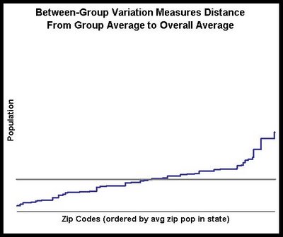
The blue slanted line is the average in each state. We see visually that much of the variation has gone away, so we would expect most variation to be within a state rather than between states.

The idea is that we measure the variation using the first approach and we measure the variation using the second approach. The ratio of these two values tells us how much of the variation is due to between-groups changes. The remaining variation must be due to within-group variation. The next section shows the calculation in SQL.

Doing the Calculation in SQL
Expressing this in SQL is simply a matter of calculating the various sums of squared differences. The following SQL statement calculates both the within-group and between-group variation:

SELECT (SUM((g.grpval - a.allval)*(g.grpval - a.allval))/
........SUM((d.val - a.allval)*(d.val - a.allval))
.......) as between_grp,
.......(SUM((d.val - g.grpval)*(d.val - g.grpval)) /
........SUM((d.val - a.allval)*(d.val - a.allval))
.......) as within_grp
FROM (SELECT state as grp, population as val
......FROM censusfiles.zipcensus zc
.....) d JOIN
.....(SELECT state as grp, AVG(population) as grpval
......FROM censusfiles.zipcensus zc
......GROUP BY 1
.....) g
.....ON d.grp = g.grp CROSS JOIN
.....(SELECT AVG(population) as allval
......FROM censusfiles.zipcensus zc
.....) a

First note that I snuck in the calculation for both within- and between- group variation, even though I only explained the latter.

The from clause has three subqueries. Each of these calculates one level of the summary -- the value for each zip, the value for each state, and the overall value. All the queries rename the fields to some canonical name. This means that we can change the field we are looking at and not have to modify the outer SELECT clause -- a convenience that reduces the chance of error.

In addition, the structure of the query makes it fairly easy to use a calculated field rather than just a column. The same calculation would need to be used for all the fields.

And finally, if you are using a database that supports window functions -- such as SQL Server or Oracle -- then the statement for the query can be much simpler.

Discussion of Results
The results for population say that 12.6% of the variation in zip code population is between states and 87.4% is within states. This confirms the observation that using the state averages removed much of the variation in the data. In fact, for most of the census variables, most of the variation is within states.

There are definitely exceptions to this. One interesting exception is latitutude (which specifies how far north or south something is). The within-state variation for latitude is 5.5% and the between-state is 94.5% -- quite a reversal. The scatter plot for latitude looks quite different from the scatter plot for population:


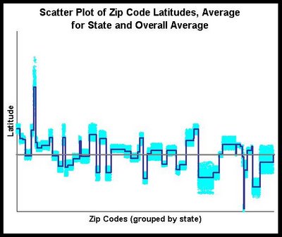
In this scatter plot, we see that the zip code values in light blue all fall quite close to the average for the state -- and in many cases, quite far from the county average. This makes a lot of sense geographically, and we see that fact both in the scatter plot and in the within-group and between-group variation.

Statistical Approach
Finally, it is instructive to go back to Paul Allison's book and look at his method for doing the same calculation in SAS. Although I am going to show SAS code, understanding the idea does not require knowing SAS -- on the other hand, it might require an advanced degree in statistics.

His proposed method is to run the following statement:

proc glm data=censusfiles.zipcensus;
....absorb state;
....model population=;
run;

And, as he states, "the proportion of variation that is between [states] is just the R-squared from this regression."

This statement is called a procedure (or proc for short) in SAS. It is calling the procedure called "glm", which stands for generalized linear model. Okay, now you can see where the advanced statistics might help.

The "absorb" option creates a separate indicator for each state. However, for performance reasons, "abosrb" does not report their values. (There are other ways to do a similar calculation that do report the individual values, but they take longer to run.)

The "model" part of the statement says what model to build. In this case, the model is predicting population, but not using any input variables. Actually, it is using input variables -- the indicators for each state created on the "absorb" line.

Doing the calculation using this method has several shortcomings. First, the results are put into a text file. They cannot easily be captured into a database table or into Excel. You have to search through lots of text to find the right metric. And, you can only run one variable at a time. In the SQL method, adding more variables is just adding more calculations on the SELECT list. And the SQL method seems easier to generalize, which I might bring up in another posting.

However, the biggest shortcoming is conceptual. Understanding variation between-groups and within-groups is not some fancy statistical procedure that requires in-depth knowledge to use correctly. Rather, it is a fundamental way of understanding data, and easy to calculate using tools, such as databases, that can readily manipulate data. The method in SQL should not only perform better on large data sets (particularly using a parallel database), but it requires much less effort to understand.

The Agent Problem: Sampling From A Finite Population

A drawer is filled with socks and you remove eight of them randomly. Four are black and four are white. How confident are you in estimating the proportion of white and black socks in the drawer?

The standard statistical approach is to assume that the number of socks in the drawer is infinite, and to use the formula for the standard error of a proportion: SQRT([proportion] * [(1 - [proportion])/[number taken out]) or, more simply, SQRT(p*q/n). In this case, the standard error is SQRT(0.5*0.5/8) = 17.7%

However, this approach clearly does not work in all cases. For instance, if there are exactly eight socks in the drawer, then the sample consists of all of them. We are 100% sure that the proportion is exactly 50%.

If there are ten socks in the drawer, then the proportion of black socks ranges from 4/10 to 6/10. These extremes are within one standard error of the observed average. Or to phrase it differently, any reasonable confidence interval (80%, 90%, 95%) contains all possible values. The confidence interval is wider than what is possible.

What does this have to do with business problems? I encountered essentially the same situation when looking at the longitudinal behavior of patients visiting physicians. I had a sample of patients who had visited the physicians and was measuring the use of a particular therapy for a particular diagnosis. Overall, about 20-30% of all patients where in the longitudinal data. And, I had pretty good estimates of the number of diagnoses for each physician.

There are several reasons why this is important. For the company that provides the therapy, knowing which physicians are using it is important. In addition, if the company does any marketing efforts, they would like to see how they perform. So, the critical question is: how well does the observed patient data characterize the physician behavior.

This is very similar to the question posed earlier. If the patient data contains eight new diagnoises and four start on the therapy of interest, how confident am I that the doctor is starting 50% of new patients on the therapy?

If there are eight patients in total, then I am 100% confident, since all of them managed to be in my sample. On the other hand, if the physician has 200 patients, then the statistical measures of standard error are more appropriate.

The situation is exacerbated by another problem. Although the longitudinal data contains 20%-30% of all patients, the distribution over the physicians is much wider. Some physicians have 10% of their patients in the data and some have 50% or more.

The solution is actually quite simple, but not normally taught in early statistics or business statistics courses. There is something called the finite population correction for exactly this situation.

[stderr-finite] = [stderr-infinite]*fpc
fpc = SQRT(([population size]- [sample size])/([population size] - 1))

So, we simply adjust the standard error and continue with whatever analysis we are using.

There is one caveat to this approach. When observed proportion is 0% or 100%, then the standard error will always be 0, even with the correction. In this case, we need to have a better estimate. In practice, I add or subtract 0.5 from the proportion to calculate the standard error.

This problem is definitely not limited to physicians and medical therapies. I think it becomes an issue in many circumstances where we want to project a global number onto smaller entities.

So, an insurance company may investigate cases for fraud. Overall, they have a large number of cases, but only 5%-10% are in the investigation. If they want to use this information to understand fraud at the agent level, then some agents will have 1% investigated and some 20%. For many of these agents, the correction factor is needed to understand our confidence in their customers' behavior.

The problem occurs because the assumption of an infinite population is reasonable over everyone. However, when we break it into smaller groups (physicians or agents), then the assumption may no longer be valid.

Statistical Test for Measuring ROI on Direct Mail Test

If I want to test the effect of return of investment on a mail/ no mail sample, however, I cannot use a parametric test since the distribution of dollar amounts do not follow a normal distribution. What non-parametric test could I use that would give me something similar to a hypothesis test of two samples?

Recently, we received an email with the question above. Since it was addressed to [email protected], it seems quite reasonable to answer it here.

First, I need to note that Michael and I are not statisticians. We don't even play one on TV (hmm, that's an interesting idea). However, we have gleaned some knowledge of statistics over the years, much from friends and colleagues who are respected statisticians.

Second, the question I am going to answer is the following: Assume that we do a test, with a test group and a control group. What we want to measure is whether the average dollars per customer is significantly different for the test group as compared to the control group. The challenge is that the dollar amounts themselve do not follow a known distribution, or the distribution is known not to be a normal distribution. For instance, we might only have two products, one that costs $10 and one that costs $100.

The reason that I'm restating the problem is because a term such as ROI (return on investment) gets thrown around a lot. In some cases, it could mean the current value of discounted future cash flows. Here, though, I think it simply means the dollar amount that customers spend (or invest, or donate, or whatever depending on the particular business).

The overall approach is that we want to measure the average and standard error for each of the groups. Then, we'll apply a simple "standard error" of the difference to see if the difference is consistently positive or negative. This is a very typical use of a z-score. And, it is a topic that I discuss in more detail in Chapter 3 of my book "Data Analysis Using SQL and Excel". In fact, the example here is slightly modified from the example in the book.

A good place to start is the Central Limit Theorem. This is a fundamental theorem for statistics. Assume that I have a population of things -- such as customers who are going to spend money in response to a marketing campaign. Assume that I take a sample of these customers and measure an average over the sample. Well, as I take more an more samples, the distribution of the averages follows a normal distribution regardless of the original distribution of values. (This is a slight oversimplification of the Central Limit Theorem, but it captures the important ideas.)

In addition, I can measure the relationship between the characteristics of the overall population and the characteristics of the sample:

(1) The average of the sample is as good an approximation as any of the average of the overall population.

(2) The standard error on the average of the sample is the standard deviation of the overall population divided by the square root of the size of the sample. Alternatively, we can phrase this in terms of variance: the variance of the sample average is the variance of the population average divided by the size of the sample.

Well, we are close. We know the average of each sample, because we can measure the average. If we knew the standard deviation of the overall population, then we could get the standard error for each group. Then, we'd know the standard error and we would be done. Well, it turns out that:

(3) The standard deviation of the sample is as good an approximation as any for the standard deviation of the population. This is convenient!

Let's assume that we have the following scenario.

Our test group has 17,839 customers, and the overall average purchase is $85.48. The control group has 53,537 customers, and the average purchase is $70.14. Is this statistically different?

We need some additional information, namely the standard deviation for each group. For the test group, the standard deviation is $197.23. For the control group, it is $196.67.

The standard error for the two groups is then $197.23/sqrt(17,839) and $196.67/sqrt(53,537), which comes to $1.48 and $0.85, respectively.

So, now the question is: is the difference of the means ($85.48 - $70.14 = $15.34) significantly different from zero. We need another formula from statistics to calculate the standard error of the difference. This formula says that the standard error is the square root of the sums of the squares of standard errors. So the value is $1.71 = sqrt(0.85^2 + 1.48^2).

And we have arrived at a place where we can use the z-score. The difference of $15.34 is about 9 standard deviations from 0 (that is, 9*1.71 is about 15.34). It is highly, highly, highly unlikely that the difference includes 0, so we can say that the test group is significantly better than the control group.

In short, we can apply the concepts of normal distributions, even to calculations on dollar amounts. We do need to be careful and pay attention to what we are doing, but the Central Limit Theorem makes this possible. If you are interested in this subject, I do strongly recommend Data Analysis Using SQL and Excel, particularly Chapter 3.

--gordon